import numpy as np
import matplotlib.pyplot as plt
import pandas as pd
import warnings
warnings.filterwarnings('ignore')Week 04 (Clustering)
Clustering adalah metode untuk membagi populasi atau titik data ke dalam sejumlah kelompok sedemikian rupa sehingga titik data dalam kelompok yang sama lebih mirip dengan titik data lain dalam kelompok yang sama dan berbeda dengan titik data dalam kelompok lain. Pada dasarnya, ini adalah kumpulan objek berdasarkan kesamaan dan ketidaksamaan di antara mereka.
source: https://www.geeksforgeeks.org/clustering-in-machine-learning/
Dataset: https://drive.google.com/file/d/1QWrWOYx2cZyEfYLe652Aj8IMm8mlkMy9/view?usp=sharing
K-Means Clustering
K-means clustering adalah algoritma unsupervised learning yang mengelompokkan dataset yang belum dilabel ke dalam kluster yang berbeda berdasarkan kesamaan tertentu\(^{[1][2][3]}\). K-means clustering membutuhkan nilai k yang menandakan jumlah kluster yang akan dibentuk\(^{[1][4]}\). K-means clustering berusaha untuk meminimalisasi variasi antar kluster dan memaksimalisasi variasi antar kluster\(^{[2][5]}\). K-means clustering menggunakan rata-rata dan jarak antara data dan centroid untuk menentukan kluster\(^{[2][5]}\). K-means clustering bekerja dengan baik jika kluster memiliki bentuk bola\(^{[3]}\).
source:
[1] https://www.trivusi.web.id/2022/06/algoritma-kmeans-clustering.html
[2] https://raharja.ac.id/2020/04/19/k-means-clustering/
[3] https://ichi.pro/id/k-means-clustering-algoritma-aplikasi-metode-evaluasi-dan-kelemahan-186933724886154
[4] https://dqlab.id/k-means-clustering-salah-satu-contoh-teknik-analisis-data-populer
[5] https://sis.binus.ac.id/2022/01/31/clustering-algoritma-k-means/.
Importing the libraries
Importing the dataset
dataset = pd.read_csv('Mall_Customers.csv')
dataset| CustomerID | Genre | Age | Annual Income (k$) | Spending Score (1-100) | |
|---|---|---|---|---|---|
| 0 | 1 | Male | 19 | 15 | 39 |
| 1 | 2 | Male | 21 | 15 | 81 |
| 2 | 3 | Female | 20 | 16 | 6 |
| 3 | 4 | Female | 23 | 16 | 77 |
| 4 | 5 | Female | 31 | 17 | 40 |
| ... | ... | ... | ... | ... | ... |
| 195 | 196 | Female | 35 | 120 | 79 |
| 196 | 197 | Female | 45 | 126 | 28 |
| 197 | 198 | Male | 32 | 126 | 74 |
| 198 | 199 | Male | 32 | 137 | 18 |
| 199 | 200 | Male | 30 | 137 | 83 |
200 rows × 5 columns
X = dataset.iloc[:, [3, 4]].values
X
array([[ 15, 39],
[ 15, 81],
[ 16, 6],
[ 16, 77],
[ 17, 40],
[ 17, 76],
[ 18, 6],
[ 18, 94],
[ 19, 3],
[ 19, 72],
[ 19, 14],
[ 19, 99],
[ 20, 15],
[ 20, 77],
[ 20, 13],
[ 20, 79],
[ 21, 35],
[ 21, 66],
[ 23, 29],
[ 23, 98],
[ 24, 35],
[ 24, 73],
[ 25, 5],
[ 25, 73],
[ 28, 14],
[ 28, 82],
[ 28, 32],
[ 28, 61],
[ 29, 31],
[ 29, 87],
[ 30, 4],
[ 30, 73],
[ 33, 4],
[ 33, 92],
[ 33, 14],
[ 33, 81],
[ 34, 17],
[ 34, 73],
[ 37, 26],
[ 37, 75],
[ 38, 35],
[ 38, 92],
[ 39, 36],
[ 39, 61],
[ 39, 28],
[ 39, 65],
[ 40, 55],
[ 40, 47],
[ 40, 42],
[ 40, 42],
[ 42, 52],
[ 42, 60],
[ 43, 54],
[ 43, 60],
[ 43, 45],
[ 43, 41],
[ 44, 50],
[ 44, 46],
[ 46, 51],
[ 46, 46],
[ 46, 56],
[ 46, 55],
[ 47, 52],
[ 47, 59],
[ 48, 51],
[ 48, 59],
[ 48, 50],
[ 48, 48],
[ 48, 59],
[ 48, 47],
[ 49, 55],
[ 49, 42],
[ 50, 49],
[ 50, 56],
[ 54, 47],
[ 54, 54],
[ 54, 53],
[ 54, 48],
[ 54, 52],
[ 54, 42],
[ 54, 51],
[ 54, 55],
[ 54, 41],
[ 54, 44],
[ 54, 57],
[ 54, 46],
[ 57, 58],
[ 57, 55],
[ 58, 60],
[ 58, 46],
[ 59, 55],
[ 59, 41],
[ 60, 49],
[ 60, 40],
[ 60, 42],
[ 60, 52],
[ 60, 47],
[ 60, 50],
[ 61, 42],
[ 61, 49],
[ 62, 41],
[ 62, 48],
[ 62, 59],
[ 62, 55],
[ 62, 56],
[ 62, 42],
[ 63, 50],
[ 63, 46],
[ 63, 43],
[ 63, 48],
[ 63, 52],
[ 63, 54],
[ 64, 42],
[ 64, 46],
[ 65, 48],
[ 65, 50],
[ 65, 43],
[ 65, 59],
[ 67, 43],
[ 67, 57],
[ 67, 56],
[ 67, 40],
[ 69, 58],
[ 69, 91],
[ 70, 29],
[ 70, 77],
[ 71, 35],
[ 71, 95],
[ 71, 11],
[ 71, 75],
[ 71, 9],
[ 71, 75],
[ 72, 34],
[ 72, 71],
[ 73, 5],
[ 73, 88],
[ 73, 7],
[ 73, 73],
[ 74, 10],
[ 74, 72],
[ 75, 5],
[ 75, 93],
[ 76, 40],
[ 76, 87],
[ 77, 12],
[ 77, 97],
[ 77, 36],
[ 77, 74],
[ 78, 22],
[ 78, 90],
[ 78, 17],
[ 78, 88],
[ 78, 20],
[ 78, 76],
[ 78, 16],
[ 78, 89],
[ 78, 1],
[ 78, 78],
[ 78, 1],
[ 78, 73],
[ 79, 35],
[ 79, 83],
[ 81, 5],
[ 81, 93],
[ 85, 26],
[ 85, 75],
[ 86, 20],
[ 86, 95],
[ 87, 27],
[ 87, 63],
[ 87, 13],
[ 87, 75],
[ 87, 10],
[ 87, 92],
[ 88, 13],
[ 88, 86],
[ 88, 15],
[ 88, 69],
[ 93, 14],
[ 93, 90],
[ 97, 32],
[ 97, 86],
[ 98, 15],
[ 98, 88],
[ 99, 39],
[ 99, 97],
[101, 24],
[101, 68],
[103, 17],
[103, 85],
[103, 23],
[103, 69],
[113, 8],
[113, 91],
[120, 16],
[120, 79],
[126, 28],
[126, 74],
[137, 18],
[137, 83]])Using the elbow method to find the optimal number of clusters
help(KMeans)Help on class KMeans in module sklearn.cluster._kmeans:
class KMeans(_BaseKMeans)
| KMeans(n_clusters=8, *, init='k-means++', n_init='warn', max_iter=300, tol=0.0001, verbose=0, random_state=None, copy_x=True, algorithm='lloyd')
|
| K-Means clustering.
|
| Read more in the :ref:`User Guide <k_means>`.
|
| Parameters
| ----------
|
| n_clusters : int, default=8
| The number of clusters to form as well as the number of
| centroids to generate.
|
| init : {'k-means++', 'random'}, callable or array-like of shape (n_clusters, n_features), default='k-means++'
| Method for initialization:
|
| 'k-means++' : selects initial cluster centroids using sampling based on
| an empirical probability distribution of the points' contribution to the
| overall inertia. This technique speeds up convergence. The algorithm
| implemented is "greedy k-means++". It differs from the vanilla k-means++
| by making several trials at each sampling step and choosing the best centroid
| among them.
|
| 'random': choose `n_clusters` observations (rows) at random from data
| for the initial centroids.
|
| If an array is passed, it should be of shape (n_clusters, n_features)
| and gives the initial centers.
|
| If a callable is passed, it should take arguments X, n_clusters and a
| random state and return an initialization.
|
| n_init : 'auto' or int, default=10
| Number of times the k-means algorithm is run with different centroid
| seeds. The final results is the best output of `n_init` consecutive runs
| in terms of inertia. Several runs are recommended for sparse
| high-dimensional problems (see :ref:`kmeans_sparse_high_dim`).
|
| When `n_init='auto'`, the number of runs depends on the value of init:
| 10 if using `init='random'`, 1 if using `init='k-means++'`.
|
| .. versionadded:: 1.2
| Added 'auto' option for `n_init`.
|
| .. versionchanged:: 1.4
| Default value for `n_init` will change from 10 to `'auto'` in version 1.4.
|
| max_iter : int, default=300
| Maximum number of iterations of the k-means algorithm for a
| single run.
|
| tol : float, default=1e-4
| Relative tolerance with regards to Frobenius norm of the difference
| in the cluster centers of two consecutive iterations to declare
| convergence.
|
| verbose : int, default=0
| Verbosity mode.
|
| random_state : int, RandomState instance or None, default=None
| Determines random number generation for centroid initialization. Use
| an int to make the randomness deterministic.
| See :term:`Glossary <random_state>`.
|
| copy_x : bool, default=True
| When pre-computing distances it is more numerically accurate to center
| the data first. If copy_x is True (default), then the original data is
| not modified. If False, the original data is modified, and put back
| before the function returns, but small numerical differences may be
| introduced by subtracting and then adding the data mean. Note that if
| the original data is not C-contiguous, a copy will be made even if
| copy_x is False. If the original data is sparse, but not in CSR format,
| a copy will be made even if copy_x is False.
|
| algorithm : {"lloyd", "elkan", "auto", "full"}, default="lloyd"
| K-means algorithm to use. The classical EM-style algorithm is `"lloyd"`.
| The `"elkan"` variation can be more efficient on some datasets with
| well-defined clusters, by using the triangle inequality. However it's
| more memory intensive due to the allocation of an extra array of shape
| `(n_samples, n_clusters)`.
|
| `"auto"` and `"full"` are deprecated and they will be removed in
| Scikit-Learn 1.3. They are both aliases for `"lloyd"`.
|
| .. versionchanged:: 0.18
| Added Elkan algorithm
|
| .. versionchanged:: 1.1
| Renamed "full" to "lloyd", and deprecated "auto" and "full".
| Changed "auto" to use "lloyd" instead of "elkan".
|
| Attributes
| ----------
| cluster_centers_ : ndarray of shape (n_clusters, n_features)
| Coordinates of cluster centers. If the algorithm stops before fully
| converging (see ``tol`` and ``max_iter``), these will not be
| consistent with ``labels_``.
|
| labels_ : ndarray of shape (n_samples,)
| Labels of each point
|
| inertia_ : float
| Sum of squared distances of samples to their closest cluster center,
| weighted by the sample weights if provided.
|
| n_iter_ : int
| Number of iterations run.
|
| n_features_in_ : int
| Number of features seen during :term:`fit`.
|
| .. versionadded:: 0.24
|
| feature_names_in_ : ndarray of shape (`n_features_in_`,)
| Names of features seen during :term:`fit`. Defined only when `X`
| has feature names that are all strings.
|
| .. versionadded:: 1.0
|
| See Also
| --------
| MiniBatchKMeans : Alternative online implementation that does incremental
| updates of the centers positions using mini-batches.
| For large scale learning (say n_samples > 10k) MiniBatchKMeans is
| probably much faster than the default batch implementation.
|
| Notes
| -----
| The k-means problem is solved using either Lloyd's or Elkan's algorithm.
|
| The average complexity is given by O(k n T), where n is the number of
| samples and T is the number of iteration.
|
| The worst case complexity is given by O(n^(k+2/p)) with
| n = n_samples, p = n_features.
| Refer to :doi:`"How slow is the k-means method?" D. Arthur and S. Vassilvitskii -
| SoCG2006.<10.1145/1137856.1137880>` for more details.
|
| In practice, the k-means algorithm is very fast (one of the fastest
| clustering algorithms available), but it falls in local minima. That's why
| it can be useful to restart it several times.
|
| If the algorithm stops before fully converging (because of ``tol`` or
| ``max_iter``), ``labels_`` and ``cluster_centers_`` will not be consistent,
| i.e. the ``cluster_centers_`` will not be the means of the points in each
| cluster. Also, the estimator will reassign ``labels_`` after the last
| iteration to make ``labels_`` consistent with ``predict`` on the training
| set.
|
| Examples
| --------
|
| >>> from sklearn.cluster import KMeans
| >>> import numpy as np
| >>> X = np.array([[1, 2], [1, 4], [1, 0],
| ... [10, 2], [10, 4], [10, 0]])
| >>> kmeans = KMeans(n_clusters=2, random_state=0, n_init="auto").fit(X)
| >>> kmeans.labels_
| array([1, 1, 1, 0, 0, 0], dtype=int32)
| >>> kmeans.predict([[0, 0], [12, 3]])
| array([1, 0], dtype=int32)
| >>> kmeans.cluster_centers_
| array([[10., 2.],
| [ 1., 2.]])
|
| Method resolution order:
| KMeans
| _BaseKMeans
| sklearn.base.ClassNamePrefixFeaturesOutMixin
| sklearn.base.TransformerMixin
| sklearn.utils._set_output._SetOutputMixin
| sklearn.base.ClusterMixin
| sklearn.base.BaseEstimator
| abc.ABC
| builtins.object
|
| Methods defined here:
|
| __init__(self, n_clusters=8, *, init='k-means++', n_init='warn', max_iter=300, tol=0.0001, verbose=0, random_state=None, copy_x=True, algorithm='lloyd')
| Initialize self. See help(type(self)) for accurate signature.
|
| fit(self, X, y=None, sample_weight=None)
| Compute k-means clustering.
|
| Parameters
| ----------
| X : {array-like, sparse matrix} of shape (n_samples, n_features)
| Training instances to cluster. It must be noted that the data
| will be converted to C ordering, which will cause a memory
| copy if the given data is not C-contiguous.
| If a sparse matrix is passed, a copy will be made if it's not in
| CSR format.
|
| y : Ignored
| Not used, present here for API consistency by convention.
|
| sample_weight : array-like of shape (n_samples,), default=None
| The weights for each observation in X. If None, all observations
| are assigned equal weight.
|
| .. versionadded:: 0.20
|
| Returns
| -------
| self : object
| Fitted estimator.
|
| ----------------------------------------------------------------------
| Data and other attributes defined here:
|
| __abstractmethods__ = frozenset()
|
| __annotations__ = {'_parameter_constraints': <class 'dict'>}
|
| ----------------------------------------------------------------------
| Methods inherited from _BaseKMeans:
|
| fit_predict(self, X, y=None, sample_weight=None)
| Compute cluster centers and predict cluster index for each sample.
|
| Convenience method; equivalent to calling fit(X) followed by
| predict(X).
|
| Parameters
| ----------
| X : {array-like, sparse matrix} of shape (n_samples, n_features)
| New data to transform.
|
| y : Ignored
| Not used, present here for API consistency by convention.
|
| sample_weight : array-like of shape (n_samples,), default=None
| The weights for each observation in X. If None, all observations
| are assigned equal weight.
|
| Returns
| -------
| labels : ndarray of shape (n_samples,)
| Index of the cluster each sample belongs to.
|
| fit_transform(self, X, y=None, sample_weight=None)
| Compute clustering and transform X to cluster-distance space.
|
| Equivalent to fit(X).transform(X), but more efficiently implemented.
|
| Parameters
| ----------
| X : {array-like, sparse matrix} of shape (n_samples, n_features)
| New data to transform.
|
| y : Ignored
| Not used, present here for API consistency by convention.
|
| sample_weight : array-like of shape (n_samples,), default=None
| The weights for each observation in X. If None, all observations
| are assigned equal weight.
|
| Returns
| -------
| X_new : ndarray of shape (n_samples, n_clusters)
| X transformed in the new space.
|
| predict(self, X, sample_weight=None)
| Predict the closest cluster each sample in X belongs to.
|
| In the vector quantization literature, `cluster_centers_` is called
| the code book and each value returned by `predict` is the index of
| the closest code in the code book.
|
| Parameters
| ----------
| X : {array-like, sparse matrix} of shape (n_samples, n_features)
| New data to predict.
|
| sample_weight : array-like of shape (n_samples,), default=None
| The weights for each observation in X. If None, all observations
| are assigned equal weight.
|
| Returns
| -------
| labels : ndarray of shape (n_samples,)
| Index of the cluster each sample belongs to.
|
| score(self, X, y=None, sample_weight=None)
| Opposite of the value of X on the K-means objective.
|
| Parameters
| ----------
| X : {array-like, sparse matrix} of shape (n_samples, n_features)
| New data.
|
| y : Ignored
| Not used, present here for API consistency by convention.
|
| sample_weight : array-like of shape (n_samples,), default=None
| The weights for each observation in X. If None, all observations
| are assigned equal weight.
|
| Returns
| -------
| score : float
| Opposite of the value of X on the K-means objective.
|
| transform(self, X)
| Transform X to a cluster-distance space.
|
| In the new space, each dimension is the distance to the cluster
| centers. Note that even if X is sparse, the array returned by
| `transform` will typically be dense.
|
| Parameters
| ----------
| X : {array-like, sparse matrix} of shape (n_samples, n_features)
| New data to transform.
|
| Returns
| -------
| X_new : ndarray of shape (n_samples, n_clusters)
| X transformed in the new space.
|
| ----------------------------------------------------------------------
| Methods inherited from sklearn.base.ClassNamePrefixFeaturesOutMixin:
|
| get_feature_names_out(self, input_features=None)
| Get output feature names for transformation.
|
| The feature names out will prefixed by the lowercased class name. For
| example, if the transformer outputs 3 features, then the feature names
| out are: `["class_name0", "class_name1", "class_name2"]`.
|
| Parameters
| ----------
| input_features : array-like of str or None, default=None
| Only used to validate feature names with the names seen in :meth:`fit`.
|
| Returns
| -------
| feature_names_out : ndarray of str objects
| Transformed feature names.
|
| ----------------------------------------------------------------------
| Data descriptors inherited from sklearn.base.ClassNamePrefixFeaturesOutMixin:
|
| __dict__
| dictionary for instance variables (if defined)
|
| __weakref__
| list of weak references to the object (if defined)
|
| ----------------------------------------------------------------------
| Methods inherited from sklearn.utils._set_output._SetOutputMixin:
|
| set_output(self, *, transform=None)
| Set output container.
|
| See :ref:`sphx_glr_auto_examples_miscellaneous_plot_set_output.py`
| for an example on how to use the API.
|
| Parameters
| ----------
| transform : {"default", "pandas"}, default=None
| Configure output of `transform` and `fit_transform`.
|
| - `"default"`: Default output format of a transformer
| - `"pandas"`: DataFrame output
| - `None`: Transform configuration is unchanged
|
| Returns
| -------
| self : estimator instance
| Estimator instance.
|
| ----------------------------------------------------------------------
| Class methods inherited from sklearn.utils._set_output._SetOutputMixin:
|
| __init_subclass__(auto_wrap_output_keys=('transform',), **kwargs) from abc.ABCMeta
| This method is called when a class is subclassed.
|
| The default implementation does nothing. It may be
| overridden to extend subclasses.
|
| ----------------------------------------------------------------------
| Methods inherited from sklearn.base.BaseEstimator:
|
| __getstate__(self)
|
| __repr__(self, N_CHAR_MAX=700)
| Return repr(self).
|
| __setstate__(self, state)
|
| get_params(self, deep=True)
| Get parameters for this estimator.
|
| Parameters
| ----------
| deep : bool, default=True
| If True, will return the parameters for this estimator and
| contained subobjects that are estimators.
|
| Returns
| -------
| params : dict
| Parameter names mapped to their values.
|
| set_params(self, **params)
| Set the parameters of this estimator.
|
| The method works on simple estimators as well as on nested objects
| (such as :class:`~sklearn.pipeline.Pipeline`). The latter have
| parameters of the form ``<component>__<parameter>`` so that it's
| possible to update each component of a nested object.
|
| Parameters
| ----------
| **params : dict
| Estimator parameters.
|
| Returns
| -------
| self : estimator instance
| Estimator instance.
from sklearn.cluster import KMeans
wcss = []
for i in range(1, 11):
    kmeans = KMeans(n_clusters = i, init = 'k-means++', random_state = 42)
    kmeans.fit(X)
    wcss.append(kmeans.inertia_)
plt.plot(range(1, 11), wcss)
plt.title('The Elbow Method')
plt.xlabel('Number of clusters')
plt.ylabel('WCSS')
plt.show()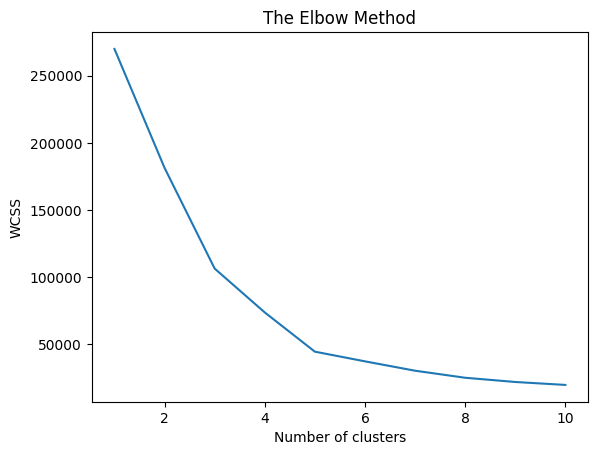
wcss[269981.28,
181363.59595959593,
106348.37306211122,
73679.78903948836,
44448.4554479337,
37233.814510710006,
30259.65720728547,
25011.839349156588,
21862.092672182895,
19672.072849014323]Within-Cluster Sum-of-Squares criterion:
\(\sum_{i=0}^{n}\min_{\mu_j \in C}(||x_i - \mu_j||^2)\)
source:
[1] https://scikit-learn.org/stable/modules/clustering.html#k-means
[2] https://stats.stackexchange.com/questions/158210/k-means-why-minimizing-wcss-is-maximizing-distance-between-clusters
Using the silhouette method to find the optimal number of clusters
Nilai Silhouette mengukur seberapa mirip sebuah titik dengan klasternya sendiri (kohesi) dibandingkan dengan klaster lain (pemisahan).
Kisaran nilai Silhouette adalah antara +1 dan -1. Nilai yang tinggi diinginkan dan mengindikasikan bahwa titik tersebut ditempatkan pada klaster yang benar. Jika banyak titik yang memiliki nilai Silhouette negatif, hal ini dapat mengindikasikan bahwa kita telah membuat terlalu banyak atau terlalu sedikit cluster.


source: https://medium.com/analytics-vidhya/how-to-determine-the-optimal-k-for-k-means-708505d204eb
import sklearn.metrics as metrics
for i in range(2,11):
  labels=KMeans(n_clusters=i,random_state=200).fit(X).labels_
  print ("Silhouette score for k(clusters) = "+str(i)+" is "+str(metrics.silhouette_score(X,labels,metric="euclidean",sample_size=1000,random_state=200)))
Silhouette score for k(clusters) = 2 is 0.2968969162503008
Silhouette score for k(clusters) = 3 is 0.46761358158775423
Silhouette score for k(clusters) = 4 is 0.4931963109249047
Silhouette score for k(clusters) = 5 is 0.553931997444648
Silhouette score for k(clusters) = 6 is 0.5379675585622219
Silhouette score for k(clusters) = 7 is 0.5367379891273258
Silhouette score for k(clusters) = 8 is 0.4592958445675391
Silhouette score for k(clusters) = 9 is 0.45770857148861777
Silhouette score for k(clusters) = 10 is 0.446735677440187Training the K-Means model on the dataset
kmeans = KMeans(n_clusters = 5, init = 'k-means++', random_state = 42)
y_kmeans = kmeans.fit_predict(X)
Visualising the clusters
plt.scatter(X[y_kmeans == 0, 0], X[y_kmeans == 0, 1], s = 100, c = 'red', label = 'Cluster 1')
plt.scatter(X[y_kmeans == 1, 0], X[y_kmeans == 1, 1], s = 100, c = 'blue', label = 'Cluster 2')
plt.scatter(X[y_kmeans == 2, 0], X[y_kmeans == 2, 1], s = 100, c = 'green', label = 'Cluster 3')
plt.scatter(X[y_kmeans == 3, 0], X[y_kmeans == 3, 1], s = 100, c = 'cyan', label = 'Cluster 4')
plt.scatter(X[y_kmeans == 4, 0], X[y_kmeans == 4, 1], s = 100, c = 'magenta', label = 'Cluster 5')
plt.scatter(kmeans.cluster_centers_[:, 0], kmeans.cluster_centers_[:, 1], s = 300, c = 'yellow', label = 'Centroids')
plt.title('Clusters of customers')
plt.xlabel('Annual Income (k$)')
plt.ylabel('Spending Score (1-100)')
plt.legend()
plt.show()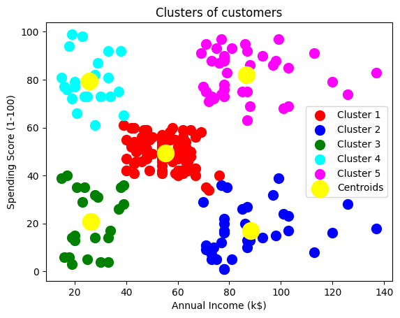
kmeans.cluster_centers_array([[55.2962963 , 49.51851852],
[88.2 , 17.11428571],
[26.30434783, 20.91304348],
[25.72727273, 79.36363636],
[86.53846154, 82.12820513]])kmeans.labels_array([2, 3, 2, 3, 2, 3, 2, 3, 2, 3, 2, 3, 2, 3, 2, 3, 2, 3, 2, 3, 2, 3,
2, 3, 2, 3, 2, 3, 2, 3, 2, 3, 2, 3, 2, 3, 2, 3, 2, 3, 2, 3, 2, 0,
2, 3, 0, 0, 0, 0, 0, 0, 0, 0, 0, 0, 0, 0, 0, 0, 0, 0, 0, 0, 0, 0,
0, 0, 0, 0, 0, 0, 0, 0, 0, 0, 0, 0, 0, 0, 0, 0, 0, 0, 0, 0, 0, 0,
0, 0, 0, 0, 0, 0, 0, 0, 0, 0, 0, 0, 0, 0, 0, 0, 0, 0, 0, 0, 0, 0,
0, 0, 0, 0, 0, 0, 0, 0, 0, 0, 0, 0, 0, 4, 1, 4, 0, 4, 1, 4, 1, 4,
0, 4, 1, 4, 1, 4, 1, 4, 1, 4, 0, 4, 1, 4, 1, 4, 1, 4, 1, 4, 1, 4,
1, 4, 1, 4, 1, 4, 1, 4, 1, 4, 1, 4, 1, 4, 1, 4, 1, 4, 1, 4, 1, 4,
1, 4, 1, 4, 1, 4, 1, 4, 1, 4, 1, 4, 1, 4, 1, 4, 1, 4, 1, 4, 1, 4,
1, 4], dtype=int32)Hierarchical Clustering
Using the dendrogram to find the optimal number of clusters
import scipy.cluster.hierarchy as sch
dendrogram = sch.dendrogram(sch.linkage(X, method = 'ward'))
plt.title('Dendrogram')
plt.xlabel('Customers')
plt.ylabel('Euclidean distances')
plt.show()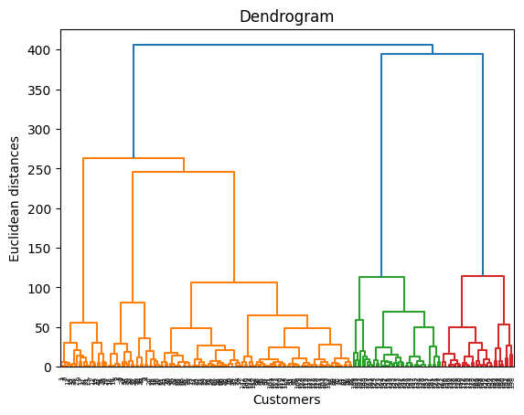
help(sch.linkage)Help on function linkage in module scipy.cluster.hierarchy:
linkage(y, method='single', metric='euclidean', optimal_ordering=False)
Perform hierarchical/agglomerative clustering.
The input y may be either a 1-D condensed distance matrix
or a 2-D array of observation vectors.
If y is a 1-D condensed distance matrix,
then y must be a :math:`\binom{n}{2}` sized
vector, where n is the number of original observations paired
in the distance matrix. The behavior of this function is very
similar to the MATLAB linkage function.
A :math:`(n-1)` by 4 matrix ``Z`` is returned. At the
:math:`i`-th iteration, clusters with indices ``Z[i, 0]`` and
``Z[i, 1]`` are combined to form cluster :math:`n + i`. A
cluster with an index less than :math:`n` corresponds to one of
the :math:`n` original observations. The distance between
clusters ``Z[i, 0]`` and ``Z[i, 1]`` is given by ``Z[i, 2]``. The
fourth value ``Z[i, 3]`` represents the number of original
observations in the newly formed cluster.
The following linkage methods are used to compute the distance
:math:`d(s, t)` between two clusters :math:`s` and
:math:`t`. The algorithm begins with a forest of clusters that
have yet to be used in the hierarchy being formed. When two
clusters :math:`s` and :math:`t` from this forest are combined
into a single cluster :math:`u`, :math:`s` and :math:`t` are
removed from the forest, and :math:`u` is added to the
forest. When only one cluster remains in the forest, the algorithm
stops, and this cluster becomes the root.
A distance matrix is maintained at each iteration. The ``d[i,j]``
entry corresponds to the distance between cluster :math:`i` and
:math:`j` in the original forest.
At each iteration, the algorithm must update the distance matrix
to reflect the distance of the newly formed cluster u with the
remaining clusters in the forest.
Suppose there are :math:`|u|` original observations
:math:`u[0], \ldots, u[|u|-1]` in cluster :math:`u` and
:math:`|v|` original objects :math:`v[0], \ldots, v[|v|-1]` in
cluster :math:`v`. Recall, :math:`s` and :math:`t` are
combined to form cluster :math:`u`. Let :math:`v` be any
remaining cluster in the forest that is not :math:`u`.
The following are methods for calculating the distance between the
newly formed cluster :math:`u` and each :math:`v`.
* method='single' assigns
.. math::
d(u,v) = \min(dist(u[i],v[j]))
for all points :math:`i` in cluster :math:`u` and
:math:`j` in cluster :math:`v`. This is also known as the
Nearest Point Algorithm.
* method='complete' assigns
.. math::
d(u, v) = \max(dist(u[i],v[j]))
for all points :math:`i` in cluster u and :math:`j` in
cluster :math:`v`. This is also known by the Farthest Point
Algorithm or Voor Hees Algorithm.
* method='average' assigns
.. math::
d(u,v) = \sum_{ij} \frac{d(u[i], v[j])}
{(|u|*|v|)}
for all points :math:`i` and :math:`j` where :math:`|u|`
and :math:`|v|` are the cardinalities of clusters :math:`u`
and :math:`v`, respectively. This is also called the UPGMA
algorithm.
* method='weighted' assigns
.. math::
d(u,v) = (dist(s,v) + dist(t,v))/2
where cluster u was formed with cluster s and t and v
is a remaining cluster in the forest (also called WPGMA).
* method='centroid' assigns
.. math::
dist(s,t) = ||c_s-c_t||_2
where :math:`c_s` and :math:`c_t` are the centroids of
clusters :math:`s` and :math:`t`, respectively. When two
clusters :math:`s` and :math:`t` are combined into a new
cluster :math:`u`, the new centroid is computed over all the
original objects in clusters :math:`s` and :math:`t`. The
distance then becomes the Euclidean distance between the
centroid of :math:`u` and the centroid of a remaining cluster
:math:`v` in the forest. This is also known as the UPGMC
algorithm.
* method='median' assigns :math:`d(s,t)` like the ``centroid``
method. When two clusters :math:`s` and :math:`t` are combined
into a new cluster :math:`u`, the average of centroids s and t
give the new centroid :math:`u`. This is also known as the
WPGMC algorithm.
* method='ward' uses the Ward variance minimization algorithm.
The new entry :math:`d(u,v)` is computed as follows,
.. math::
d(u,v) = \sqrt{\frac{|v|+|s|}
{T}d(v,s)^2
+ \frac{|v|+|t|}
{T}d(v,t)^2
- \frac{|v|}
{T}d(s,t)^2}
where :math:`u` is the newly joined cluster consisting of
clusters :math:`s` and :math:`t`, :math:`v` is an unused
cluster in the forest, :math:`T=|v|+|s|+|t|`, and
:math:`|*|` is the cardinality of its argument. This is also
known as the incremental algorithm.
Warning: When the minimum distance pair in the forest is chosen, there
may be two or more pairs with the same minimum distance. This
implementation may choose a different minimum than the MATLAB
version.
Parameters
----------
y : ndarray
A condensed distance matrix. A condensed distance matrix
is a flat array containing the upper triangular of the distance matrix.
This is the form that ``pdist`` returns. Alternatively, a collection of
:math:`m` observation vectors in :math:`n` dimensions may be passed as
an :math:`m` by :math:`n` array. All elements of the condensed distance
matrix must be finite, i.e., no NaNs or infs.
method : str, optional
The linkage algorithm to use. See the ``Linkage Methods`` section below
for full descriptions.
metric : str or function, optional
The distance metric to use in the case that y is a collection of
observation vectors; ignored otherwise. See the ``pdist``
function for a list of valid distance metrics. A custom distance
function can also be used.
optimal_ordering : bool, optional
If True, the linkage matrix will be reordered so that the distance
between successive leaves is minimal. This results in a more intuitive
tree structure when the data are visualized. defaults to False, because
this algorithm can be slow, particularly on large datasets [2]_. See
also the `optimal_leaf_ordering` function.
.. versionadded:: 1.0.0
Returns
-------
Z : ndarray
The hierarchical clustering encoded as a linkage matrix.
Notes
-----
1. For method 'single', an optimized algorithm based on minimum spanning
tree is implemented. It has time complexity :math:`O(n^2)`.
For methods 'complete', 'average', 'weighted' and 'ward', an algorithm
called nearest-neighbors chain is implemented. It also has time
complexity :math:`O(n^2)`.
For other methods, a naive algorithm is implemented with :math:`O(n^3)`
time complexity.
All algorithms use :math:`O(n^2)` memory.
Refer to [1]_ for details about the algorithms.
2. Methods 'centroid', 'median', and 'ward' are correctly defined only if
Euclidean pairwise metric is used. If `y` is passed as precomputed
pairwise distances, then it is the user's responsibility to assure that
these distances are in fact Euclidean, otherwise the produced result
will be incorrect.
See Also
--------
scipy.spatial.distance.pdist : pairwise distance metrics
References
----------
.. [1] Daniel Mullner, "Modern hierarchical, agglomerative clustering
algorithms", :arXiv:`1109.2378v1`.
.. [2] Ziv Bar-Joseph, David K. Gifford, Tommi S. Jaakkola, "Fast optimal
leaf ordering for hierarchical clustering", 2001. Bioinformatics
:doi:`10.1093/bioinformatics/17.suppl_1.S22`
Examples
--------
>>> from scipy.cluster.hierarchy import dendrogram, linkage
>>> from matplotlib import pyplot as plt
>>> X = [[i] for i in [2, 8, 0, 4, 1, 9, 9, 0]]
>>> Z = linkage(X, 'ward')
>>> fig = plt.figure(figsize=(25, 10))
>>> dn = dendrogram(Z)
>>> Z = linkage(X, 'single')
>>> fig = plt.figure(figsize=(25, 10))
>>> dn = dendrogram(Z)
>>> plt.show()
Training the Hierarchical Clustering model on the dataset
Hierarchical clustering adalah keluarga umum dari algoritma clustering yang membangun cluster bersarang dengan menggabungkan atau memisahkannya secara berurutan. Hirarki cluster ini direpresentasikan sebagai sebuah pohon (atau dendogram). Akar dari pohon adalah cluster unik yang mengumpulkan semua sampel, sedangkan daunnya adalah cluster yang hanya memiliki satu sampel.
Objek AgglomerativeClustering melakukan pengelompokan hirarkis menggunakan pendekatan dari bawah ke atas: setiap pengamatan dimulai dari klasternya sendiri, dan klaster-klaster tersebut digabungkan secara berurutan. Kriteria keterkaitan menentukan metrik yang digunakan untuk strategi penggabungan:
Ward meminimalkan jumlah perbedaan kuadrat di dalam semua cluster. Ini adalah pendekatan yang meminimalkan varians dan dalam hal ini mirip dengan fungsi objektif k-means tetapi ditangani dengan pendekatan hirarki aglomeratif.
Maximum atau complete linkage meminimalkan jarak maksimum antara pengamatan dari pasangan cluster.
Average linkage meminimalkan rata-rata jarak antara semua pengamatan dari pasangan cluster.
Single linkage meminimalkan jarak antara pengamatan terdekat dari pasangan cluster.
AgglomerativeClustering juga dapat menskalakan ke sejumlah besar sampel ketika digunakan bersama dengan matriks konektivitas, tetapi secara komputasi mahal ketika tidak ada batasan konektivitas yang ditambahkan di antara sampel: ia mempertimbangkan pada setiap langkah semua kemungkinan penggabungan.
source : https://scikit-learn.org/stable/modules/clustering.html#hierarchical-clustering
from sklearn.cluster import AgglomerativeClustering
hc = AgglomerativeClustering(n_clusters = 5, affinity = 'euclidean', linkage = 'ward')
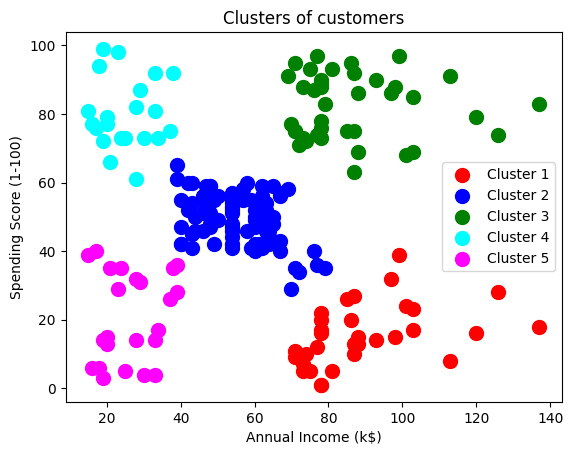
y_hc = hc.fit_predict(X)Visualising the clusters
plt.scatter(X[y_hc == 0, 0], X[y_hc == 0, 1], s = 100, c = 'red', label = 'Cluster 1')
plt.scatter(X[y_hc == 1, 0], X[y_hc == 1, 1], s = 100, c = 'blue', label = 'Cluster 2')
plt.scatter(X[y_hc == 2, 0], X[y_hc == 2, 1], s = 100, c = 'green', label = 'Cluster 3')
plt.scatter(X[y_hc == 3, 0], X[y_hc == 3, 1], s = 100, c = 'cyan', label = 'Cluster 4')
plt.scatter(X[y_hc == 4, 0], X[y_hc == 4, 1], s = 100, c = 'magenta', label = 'Cluster 5')
plt.title('Clusters of customers')
plt.xlabel('Annual Income (k$)')
plt.ylabel('Spending Score (1-100)')
plt.legend()
plt.show()